What Actually Happens Inside a Vector Database (A Tour of HNSW)

Here is a claim that sounds like a typo: your production vector database is wrong on purpose, and that is the feature you're paying for. It does not return the nearest neighbors to your query. It returns the probably-nearest ones, most of the time, precisely because returning the actually-nearest ones would be too slow to ship. Once you internalize that a vector search is a tunable accuracy/speed tradeoff, not a correctness guarantee, the whole subsystem stops being magic and becomes an index — one you tune like any other.

Let me show you what's actually happening under the hood — "it just finds similar stuff" hides all the interesting engineering.

The setup: nearest neighbor sounds trivial

Semantic search and RAG both run on the same trick. You push text — a document chunk, a product description, a user's question — through an embedding model that returns a vector: a list of floats, usually 768 to 3072 dimensions depending on the model. The geometry is the point. Texts that mean similar things land close together in that high-dimensional space; different meanings land far apart. "Close" is cosine similarity, dot product, or L2 (Euclidean) distance — for normalized vectors, basically interchangeable.

So retrieval reduces to one operation: given a query vector, find the k nearest vectors in your collection. That's it — the whole job of a vector index.

And it sounds trivial because at small scale it is trivial. The trouble hides in "in your collection." At ten thousand vectors, nearest-neighbor is a homework problem. At a hundred million vectors and thousands of queries per second, it becomes the single most expensive thing your service does, and the naive answer stops working entirely.

Brute force: correct, and doomed

The obvious algorithm is exact, and has many names — brute force, flat index, exact kNN. Take the query vector, compare it against every vector in the collection, sort by distance, return the top k.

This is genuinely perfect. It has 100% recall by definition: it looked at everything, so it cannot miss.

The cost is where it dies. Every query is O(N·d) — for each of N vectors, a d-dimensional distance computation. At N = 10,000 and d = 768 that's a few million multiply-adds, which a CPU shrugs off in milliseconds. At N = 100,000,000 and d = 1536 it's over a hundred billion multiply-adds per query — then multiply by your QPS. The work scales linearly with the dataset, forever, and no caching saves you, because every query lands somewhere new.

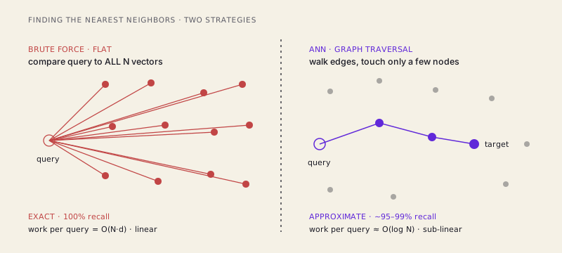
This is the concrete reason you cannot just add a vector column to Postgres, write ORDER BY embedding <-> query LIMIT 10, and call it a semantic search engine. That's a sequential scan over the whole table, a distance calc on every row — correct, fine for your demo, and it melts the moment real traffic and real data arrive. Flat indexes fit tens of thousands of vectors, not millions.

The trade: give up exactness, buy back speed

Here's the move that makes vector search at scale possible: stop insisting on the exact nearest neighbors. This is Approximate Nearest Neighbor search, ANN, the deal at the heart of every serious vector index. You accept an algorithm that returns the true nearest neighbors most of the time, and in exchange get 10–100x speedups, sometimes far more.

The quality metric for how good a deal you're getting is recall@k: of the true top-k nearest neighbors, what fraction did the index actually return? A recall of 0.98 means you're getting, on average, 9.8 of the real top 10 and quietly substituting a slightly-worse neighbor for the last one. For semantic search feeding an LLM, that's almost always invisible — the 10th-best chunk versus the 11th changes nothing about the answer. So you trade it for an order of magnitude less compute.

The mental model to lock in: a vector search is a dial, not a fact. One end is slow and exact, the other fast and approximate. You pick where you sit, per query — and running a vector database is just choosing that point deliberately instead of by accident.

HNSW: the graph that ate the industry

The dominant way to build that dial is a graph index called HNSW — Hierarchical Navigable Small World. If you've used pgvector, Qdrant, Weaviate, Milvus, Elasticsearch, Lucene, or FAISS, you've very likely used HNSW; it's the default in most of them for good reason. The name is a mouthful, so let's build the intuition it's made of.

Start with a plain proximity graph. Every vector is a node, connected by edges to some of its nearest neighbors. To search, start at some node, look at its neighbors, and hop to whichever one is closest to your query. Repeat from the new node, walking "downhill" toward the query until no neighbor is closer than where you're standing. That greedy walk is the core idea, and on a well-connected graph it converges on the query's neighborhood without touching most of the collection.

The problem with a single flat graph: greedy walks get stuck and take too many hops when the entry point is far from the target. HNSW's fix is the "hierarchical" part, borrowed straight from the skip list — the classic structure that stacks express lanes on a linked list so you skip ahead instead of trudging node by node.

HNSW stacks layers of graphs. The bottom layer, layer 0, contains every node, densely connected to its local neighbors — short-range links. Each layer above is sparser: a random subset of the nodes with longer-range links, the express lanes that cross the space in a few big jumps. A node's top layer is assigned randomly on insert, with exponentially decaying probability — almost all nodes live only at the bottom, a few reach one level up, a handful higher, exactly like tower heights in a skip list generalized to a graph.

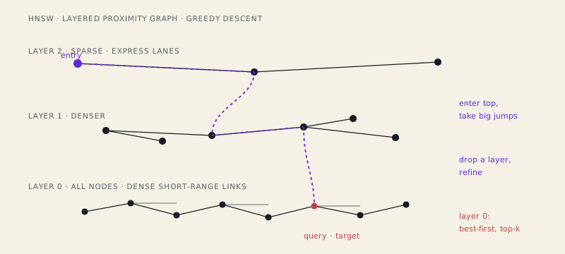
Now the search. You enter at the single entry point on the top, sparsest layer and greedily walk toward the query until no neighbor there is closer. Because the top layer's edges are long, those few hops cover enormous distance — you've crossed the space cheaply. Then you drop down a layer, using your current best node as the new starting point, and greedily walk again on that denser graph. You repeat, descending layer by layer, each adding local detail, until you reach layer 0. There you do a more thorough best-first search — keeping a candidate list of promising nodes rather than a single current-best — and return the top k.

The payoff is the whole reason HNSW exists: roughly O(log N) hops instead of O(N) comparisons. The express lanes skip past the vast majority of the collection, spending distance computations only near the answer. That's the 100x — why a graph index answers in a millisecond what brute force needs a full scan for.

The three knobs that decide everything

HNSW's real gift is that the accuracy/speed/memory tradeoff isn't hidden — it's three parameters. Learn them and you can operate the thing.

M — max edges per node. How connected the graph is. Higher M means more paths through it: better recall and more robust search, but more memory and slower builds. Typical values are 16 to 64, fixed at build time.

efConstruction — candidate list size during build. When inserting a node, HNSW searches for its best neighbors to link to; efConstruction is how hard it looks. Higher means a higher-quality graph with better-chosen edges, lifting the recall ceiling you can later reach — at the cost of slower indexing. Also fixed at build time.

efSearch — candidate list size during query. The star. At query time, efSearch (often just ef) sets how many candidates the bottom-layer search keeps in flight. Larger ef explores more of the graph before answering: higher recall, higher latency. Smaller ef: faster, lower recall. Crucially, you can change it per query without rebuilding anything. It's the live runtime dial — turn it up for 99% recall on a high-stakes query, loosen it for raw throughput.

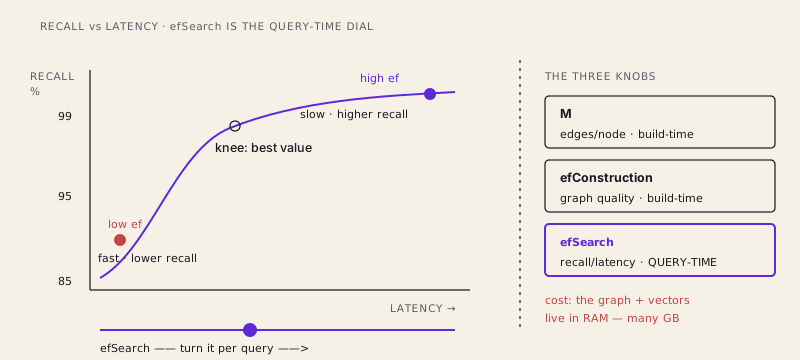
The shape to remember: recall rises fast with ef at first, then flattens into diminishing returns. Going from 90% to 98% recall is cheap; squeezing out the last fraction of a percent costs disproportionate latency. Most teams find the knee of that curve and stay there.

The honest costs

HNSW is the default because it's fast and accurate, but it's not free — the bills come due in ways worth knowing before you commit.

It's memory-hungry, and this is the big one. Graph edges and raw vectors typically live in RAM for search to be fast. A hundred million 1536-dimension float32 vectors is about 600 GB of raw vectors alone — before the graph's edges on top. Memory, not CPU, usually dominates the cost of a large HNSW deployment — it's why "just index everything" hits a wall measured in dollars per gigabyte of RAM.

Builds are slow compared to a flat index — you're constructing a whole multi-layer graph node by node — and deletes are awkward. You can't cleanly cut a node from a proximity graph without degrading it, so most implementations use tombstones (mark-as-deleted and skip) and periodically rebuild to reclaim space. A churn-heavy collection fights the data structure.

Which is why HNSW isn't the only game in town. IVF (inverted file index) takes a different tack: cluster the vectors into cells during a training step, and at query time search only the few cells nearest the query — nprobe, the number of cells to probe, is IVF's dial, trading recall for speed just like ef does. IVF is lighter on memory and cheaper to build, at the cost of that training step and generally a bit less recall-per-speed than HNSW. And quantization is the memory lever underneath all of it: product quantization (IVF-PQ), scalar, or binary quantization compress each vector down from 32-bit floats to something far smaller, fitting many more vectors in RAM in exchange for some recall. When someone fits a billion vectors on one machine, quantization is how.

The takeaway: it's just an index

Strip away the "AI" framing and a vector index is a database index with one extra axis. A B-tree trades write cost and space for fast range and equality lookups. A hash index trades ordering for O(1) point lookups. An HNSW index trades memory and build time for fast nearest-neighbor lookups — plus a recall axis the others don't have, because it's allowed to be approximately right. Choosing M, efConstruction, and efSearch is the same discipline as picking your index type and fill factor: a point in a tradeoff space, chosen on purpose.

One last thing, because it bites people: filtered search. Real queries want "nearest neighbors where tenant_id = 42 and status = 'active'," combining a metadata filter with the vector search. This is genuinely hard: the graph was built for pure geometric proximity and knows nothing about your filter — filter too aggressively and the greedy walk wanders where almost everything is filtered out, tanking recall or latency. Every serious vector DB has its own strategy (pre-filter, post-filter, filtered traversal), and it's the first place a naive setup surprises you in production.

But that's a detail on the core idea, which is simpler than the acronyms make it sound: embed into vectors, find the nearest ones, and — because exact "nearest" is too expensive at scale — walk a clever layered graph that finds them approximately, on a dial you control. That dial is the whole thing. Learn to turn it, and the vector database stops being a black box and becomes just another index you tune.